Fractal Analysis of Coral Colonies
Distinguishing coral species with today's rigid taxonomy is a frontline reef-conservation problem. We propose a continuous trait — fractal dimension — and a toolkit to compute it.
In recent years, rapid coral bleaching and extinction have driven huge conservation efforts around endangered reefs — which provide habitat, shelter, and nursing grounds for a wide range of marine life. But these efforts are often hampered by the most basic issue of all: telling different coral species apart.
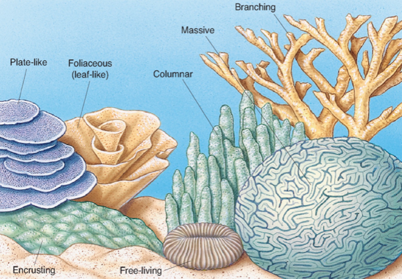
The current method relies on researchers first sorting corals into discrete categories based on skeletal features (morphological traits), then identifying the species within a category. The trouble shows up at step one, because the morphological approach doesn't account for a single species having more than one trait, nor for traits that shift with the environment (phenotypic plasticity). Misidentification — and the miscommunication it causes downstream — comes from:
- High phenotypic plasticity: one species can take on different morphologies depending on its environment, so it ends up sorted into different families.
- Crossbreeding: different "families" can interbreed, producing corals with mixed traits that don't fit predefined categories.
This work tackles the challenge of capturing a colony's structural complexity by proposing a promising continuous trait — fractal dimension — along with a toolkit to calculate it, giving researchers a reliable way to describe and differentiate coral colonies.
Why fractal dimension
Fractal geometry describes repeating patterns within a shape or structure. To quote Benoit Mandelbrot, the father of the field, a fractal is a "rough or fragmented geometric shape that can be split into parts, each of which is (at least approximately) a reduced-size copy of the whole." Nature, full of irregular forms, obeys fractal geometry surprisingly often — many natural objects can't be described cleanly by classical geometry.
Take a tree: as it grows, it splits into smaller and smaller branches, a self-similar pattern visible from the trunk down to the tiniest twig. Many fields already use fractal analysis — describing ecological systems, insect movement, image processing, chaotic trajectories, and even the branching of arteries.
Fractal dimension
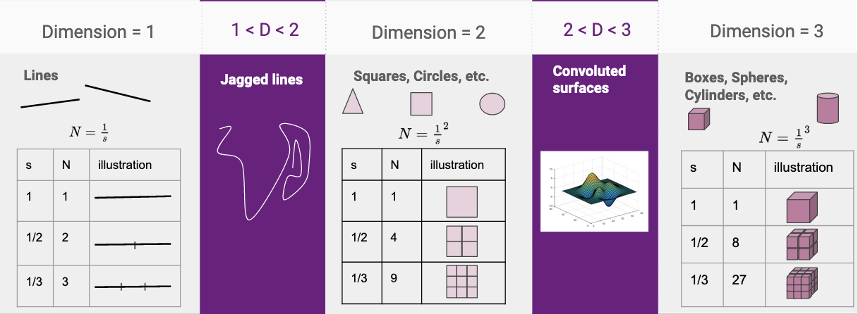
In fractal geometry, D characterizes the structural complexity of a fractal. We can build intuition from familiar dimensions: an ideal line has D = 1, an ideal plane has D = 2, an ideal space has D = 3. But a jagged line occupies a non-integer dimension somewhere between 1 (barely irregular) and 2 (highly irregular); the same logic applies to a convoluted surface.
Formally, the number of self-similar pieces N relates to the scale s by:

Fractal dimension has real advantages over traditional measures. It is:
- Orientation invariant
- Scale invariant
- Highly sensitive to structural changes in the object
That means no re-scaling or re-orienting is needed before comparing colonies.
Calculation method
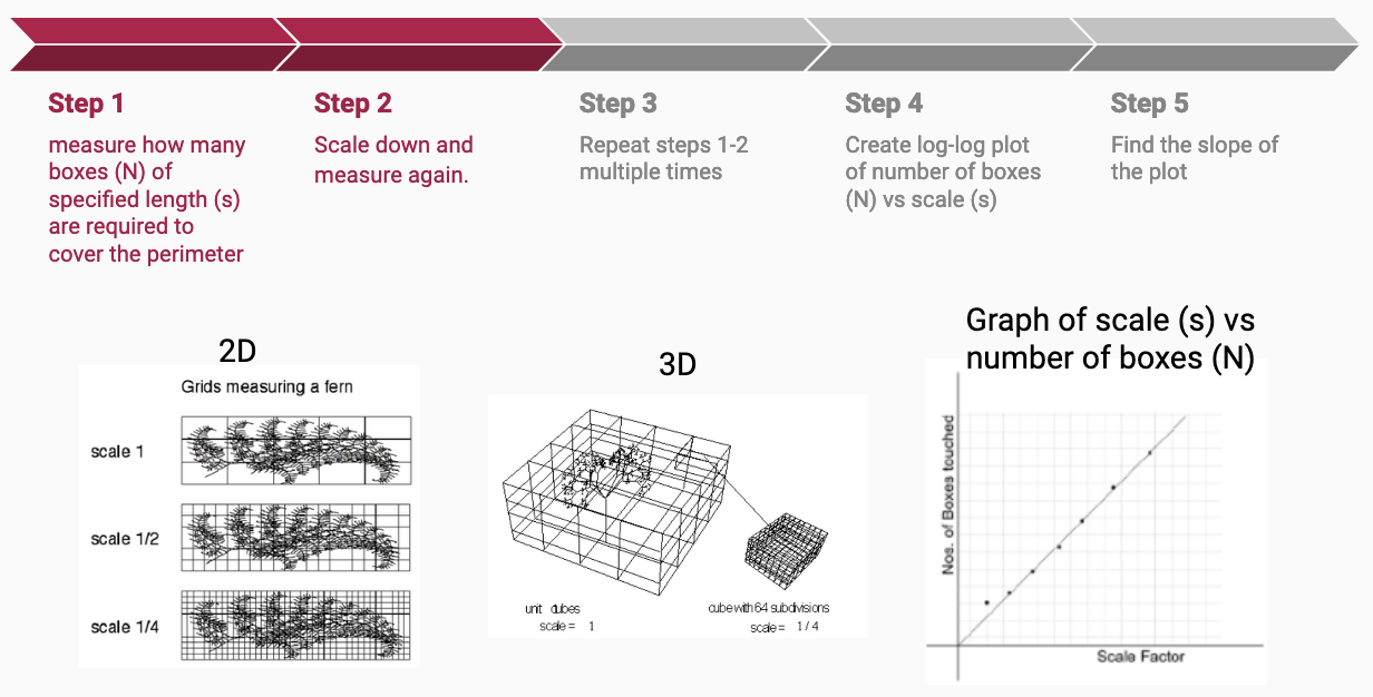
The two most common methods are Bouligand–Minkowski and cube counting. We use cube counting, where the fractal dimension is defined as:

In practice, that breaks down into a few steps:
- Measure how many boxes (N) of a given side length (s) are needed to cover the structure.
- Shrink s and measure again.
- Repeat across several scales.
- Build a log-log plot of N versus s.
- The slope of the fitted line is the fractal dimension D.
Materials & methods
We used 3D scans of 289 corals from the NTU Coral Museum, compiled into .obj files. The method has three steps: clean the .obj files, run cube counting and collect data, then analyze.
Because the corals come in fragmented pieces, some surfaces face inward rather than out at the environment. Those smooth broken surfaces don't describe the coral's true structure, so we removed them. Since fractal dimension is rotation- and scale-invariant, no normalization or reorientation was necessary. Our Python cube-counting program places the 3D object in a grid of boxes of length s, counts boxes containing vertices, repeats across lengths, plots log(s) vs log(N), fits a line, and reads D off the slope. It also reports surface area, volume, and bounding dimensions for each colony.
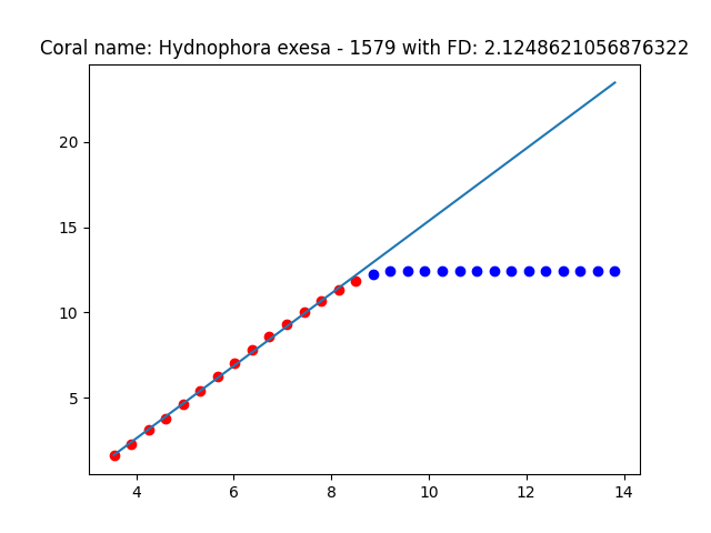
Results
The results section is still under construction — we received reviewer feedback we're eager to fold in. Check back for the updated version.
Keep reading
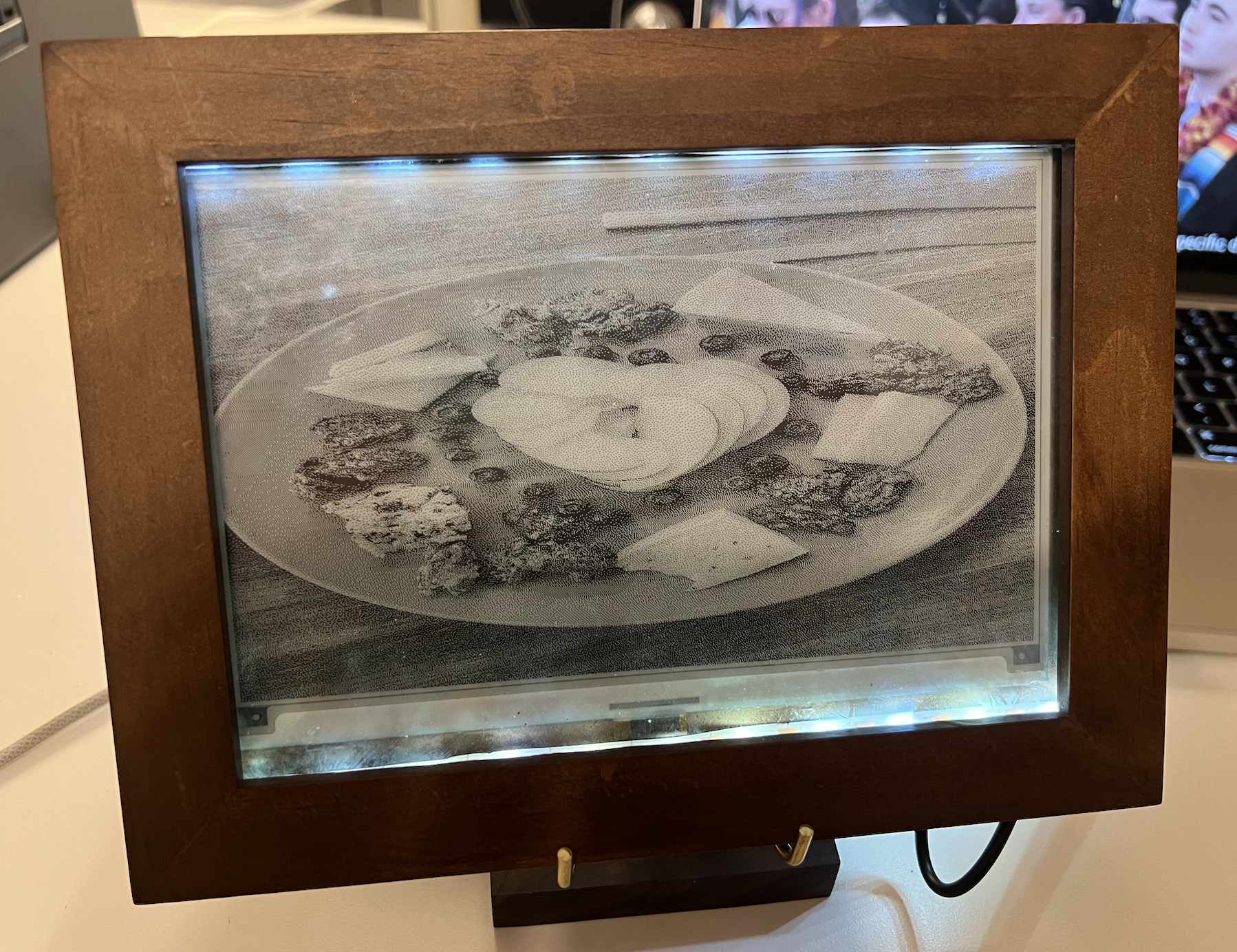
Building an E-Paper Digital Picture Frame
A low-power digital picture frame built on a Raspberry Pi and a 7.5" e-paper display. It auto-syncs photos from Google Drive, refreshes hourly, and boots straight into slideshow mode.

Launching the Allegris Seatmap
As Product Manager on the Gordian team, I helped lead the €2.5B Allegris seatmap rollout for Lufthansa — a major cabin overhaul focused on luxury and personalization.

Droneye: System Design
The system design of my year-long senior capstone: an autonomous, low-cost drone system that humanely diverts mammalian pests like squirrels and possums from backyards.